02-intro-to-r

Author

Affiliation

Professor Shannon Ellis

UC San Diego
COGS 137 - Fall 2026

Published

September 30, 2026

Introduction to R

Q&A

Q: What are some other important functions in R that we should keep in mind?

We’ll get to these today and Monday! The most important will be the verbs in the tidyverse - on Monday!

Q: Does Quarto take in / print code? Or is it primarily used just for text-based content?

It will display code as well as execute it on render. It’s for text and code.

Q: I’m curious about how we’ll be able to manipulate datasets using R, or if this is something we will end up doing. I wonder how using R will compare to using excel.

In lots of ways, Excel can do many of the things you can do with data in R; however, R has the advantage of being reproducible. This means you write the code once, but can execute it as many times as you want. This is unlike Excel, where each time you want to do something, you have to point/click to make it happen. And, there’s not a record of what’s been done, so being able to reproduce what someone else has done is nontrivial.

Q: I think I was confused as to the use of Quarto when we were running code on the console of Rstudio but I understood how Quarto is used as a source to save code, but im curious as to why the console was not made to save it.

Technically you can save your console, but for our purposes we’re not going to because it’s not particularly readable. Think of the console as a place to try things out, but anything you really want to save/keep/organize should go in a (quarto) document

Course Announcements

Due Dates:

🔘 Student survey (#finaid) due Fri 10/2 (11:59 PM)
⌨Lab 01 is due Friday - repos are available for those whose GitHub names I have
- if no lab01 available on GH, please either complete pre-course survey or email me (sellis@ucsd.edu) your GitHub username
- first lab is tomorrow (Th 5P)!
🔘 Lecture Participation survey “due” after class

Agenda

Variables
Operators
Data in R

Variables & Assignment

Variables are how we store information so that we can access it later.

. . .

Variables are created and stored using the assignment operator <-

first_variable <- 3

The above stores the value 3 in the variable first_variable

. . .

Note: Other programming languages use = for assignment. R also uses that for assignment, but it is more typical to see <- in R code, so we’ll stick with that.

. . .

This means that if we ever want to reference the information stored in that variable later, we can “call” (mean, type in our code) the variable’s name:

first_variable

[1] 3

Variable Type

Every variable you create in R will be of a specific type.

. . .

R is dynamically typed: you don’t declare a type ahead of time. R sets the type when you assign a value (and the type can change if you reassign the variable).

. . .

Determining the type of a variable with class():

class(first_variable)

[1] "numeric"

Basic Variable Types

Variable Type	Explanation	Example
character	stores a string	`"cogs137"`, `"hi!"`
numeric	stores whole numbers and decimals	`9`, `9.29`
integer	specifies integer	`9L` (the `L` specifies this is an integer)
logical	Booleans	`TRUE`, `FALSE`
list	store multiple elements	`list(7, "a", TRUE)`

Note: There are many more. We’ll get to some but not all in this course.

logical & character

logical - Boolean values TRUE and FALSE

class(TRUE)

[1] "logical"

. . .

character - character strings

class("hello")

[1] "character"

class('students') # equivalent...but we'll use double quotes!

[1] "character"

. . .

numeric: double & integer

double - floating point numerical values (default numerical type)

class(1.335)

[1] "numeric"

class(7)

[1] "numeric"

. . .

integer - integer numerical values (indicated with an L)

class(7L)

[1] "integer"

. . .

vectors

The most basic data structure in R is the vector: an ordered collection of values that are all the same type.

c(1, 2, 3)                      # combine values with c()

[1] 1 2 3

1:5                             # shortcut for a sequence of integers

[1] 1 2 3 4 5

my_letters <- c("a", "b", "c")
length(my_letters)

[1] 3

class(my_letters)

[1] "character"

. . .

A single value like 3 is just a vector of length 1.

lists

So far, every variable has been an atomic vector: it can hold many values, but they must all be the same type.

. . .

Lists are 1d objects that can contain any combination of R objects – including values of different types

mylist <- list("A", 7L, TRUE, 18.4)
mylist

[[1]]
[1] "A"

[[2]]
[1] 7

[[3]]
[1] TRUE

[[4]]
[1] 18.4

str(mylist)

List of 4
 $ : chr "A"
 $ : int 7
 $ : logi TRUE
 $ : num 18.4

Your Turn

Define variables of each of the following types: character, numeric, integer, logical, list

Put a green sticky on the front of your computer when you’re done. Put a pink if you want help/have a question.

Functions

class() (and View() & median()) were our first functions…but we’ll show a few more.

. . .

Functions are (most often) verbs, followed by what they will be applied to in parentheses.

. . .

Functions are:

available from base R
available from packages you import
defined by you

Helpful Functions

class() - determine high-level variable type

class(mylist)

[1] "list"

length()- determine how long an object is

# contains 4 elements
length(mylist)

[1] 4

str() - display the structure of an R object

str(mylist)

List of 4
 $ : chr "A"
 $ : int 7
 $ : logi TRUE
 $ : num 18.4

Coercion

A vector can only hold one type. If you combine different types, R coerces (converts) them to a common type – without any warning.

(This is separate from dynamic typing, which is about how a variable gets its type.)

. . .

🤔 Predict: What will each of these return?

c(1, "Hello")
c(FALSE, 3L)
c(1.2, 3L)

Put a green sticky on the front of your computer when you have your predictions.

Coercion: Answers

c(1, "Hello")

[1] "1"     "Hello"

c(FALSE, 3L)

[1] 0 3

c(1.2, 3L)

[1] 1.2 3.0

. . .

R converts to the most flexible type needed:

logical → integer → double → character

Missing Values

R uses NA to represent missing values in its data structures.

class(NA)

[1] "logical"

. . .

NA is “contagious”: most calculations involving NA return NA…

mean(c(1, 2, NA))

[1] NA

. . .

…unless you tell R to remove missing values first:

mean(c(1, 2, NA), na.rm = TRUE)

[1] 1.5

Other Special Values

NaN | Not a number

0 / 0

[1] NaN

Inf | Positive infinity

1 / 0

[1] Inf

-Inf | Negative infinity

-1 / 0

[1] -Inf

Operators

At its simplest, R is a calculator. To carry out mathematical operations, R uses operators.

Arithmetic Operators

Operator	Description
`+`	addition
`-`	subtraction
`*`	multiplication
`/`	division
`^` or `**`	exponentiation
`x %% y`	modulus (x mod y) `9%%2` is 1
`x %/% y`	integer division `9%/%2` is 4

Arithmetic Operators: Examples

7 + 6

[1] 13

2 - 3

[1] -1

4 * 2

[1] 8

9 / 2

[1] 4.5

Reminder

Output can be stored to a variable

my_addition <- 7 + 6

. . .

my_addition

[1] 13

Comparison Operators

These operators return a Boolean.

Operator	Description
`<`	less than
`<=`	less than or equal to
`>`	greater than
`>=`	greater than or equal to
`==`	exactly equal to
`!=`	not equal to

Comparison Operators: Examples

4 < 12

[1] TRUE

4 >= 3

[1] TRUE

6 == 6

[1] TRUE

7 != 6

[1] TRUE

Logical Operators

Combine (or negate) TRUE/FALSE values. You’ll use these constantly to filter data.

& and: TRUE only if both sides are TRUE
| or: TRUE if either side is TRUE
! not: flips TRUE ↔︎ FALSE

(4 < 12) & (6 == 6)

[1] TRUE

(4 > 12) | (6 == 6)

[1] TRUE

!(6 == 6)

[1] FALSE

Your Turn

Store your age (in years) in the variable my_age.
Use arithmetic to calculate (roughly) how many days old you are. Store it in days_old.
Use comparison and logical operators to check whether days_old is between 7,000 and 10,000.

Put a green sticky on the front of your computer when you’re done. Put a pink if you want help/have a question.

R Packages

Packages

Install a package once per computer with install.packages()
Load it in every session (and at the top of every Quarto document that uses it) with library()

install.packages("package_name")   # once
library(package_name)              # every time

. . .

Think of it like an app: you install it once, but you open it every time you want to use it.

. . .

In this course, most packages we’ll use have been installed for you already on datahub, so you will only have to load the package in (using library).

. . .

Question

Should install.packages() go in your Quarto document or in the console? Why?

Hint: Think back to our discussion on the first day about what the console is for vs. what a Quarto document is for…and what happens every time you render.

Data “sets”

Data “sets” in R

“set” is in quotation marks because it is not a formal data class
A tidy data “set” can be one of the following types:
- tibble
- data.frame
We’ll often work with tibbles:
- readr package (e.g. read_csv function) loads data as a tibble by default
- tibbles are part of the tidyverse, so they work well with other packages we are using
- they make minimal assumptions about your data, so are less likely to cause hard to track bugs in your code

Data frames

A data frame is the most commonly used data structure in R, they are list of equal length vectors (usually atomic, but can be generic). Each vector is treated as a column and elements of the vectors as rows.
A tibble is a type of data frame that … makes your life (i.e. data analysis) easier.
Most often a data frame will be constructed by reading in from a file, but we can create them from scratch.

df <- tibble(x = 1:3, y = c("a", "b", "c"))
class(df)

[1] "tbl_df"     "tbl"        "data.frame"

glimpse(df)

Rows: 3
Columns: 2
$ x <int> 1, 2, 3
$ y <chr> "a", "b", "c"

Data frames (cont.)

Columns (variables) in data frames are accessed with $:

dataframe$var_name

. . .

class(df$x)  # access variable type for column

[1] "integer"

class(df$y)

[1] "character"

Variable Types

Data stored in columns can include different kinds of information…which would require a different type (class) of variable to be used in R.

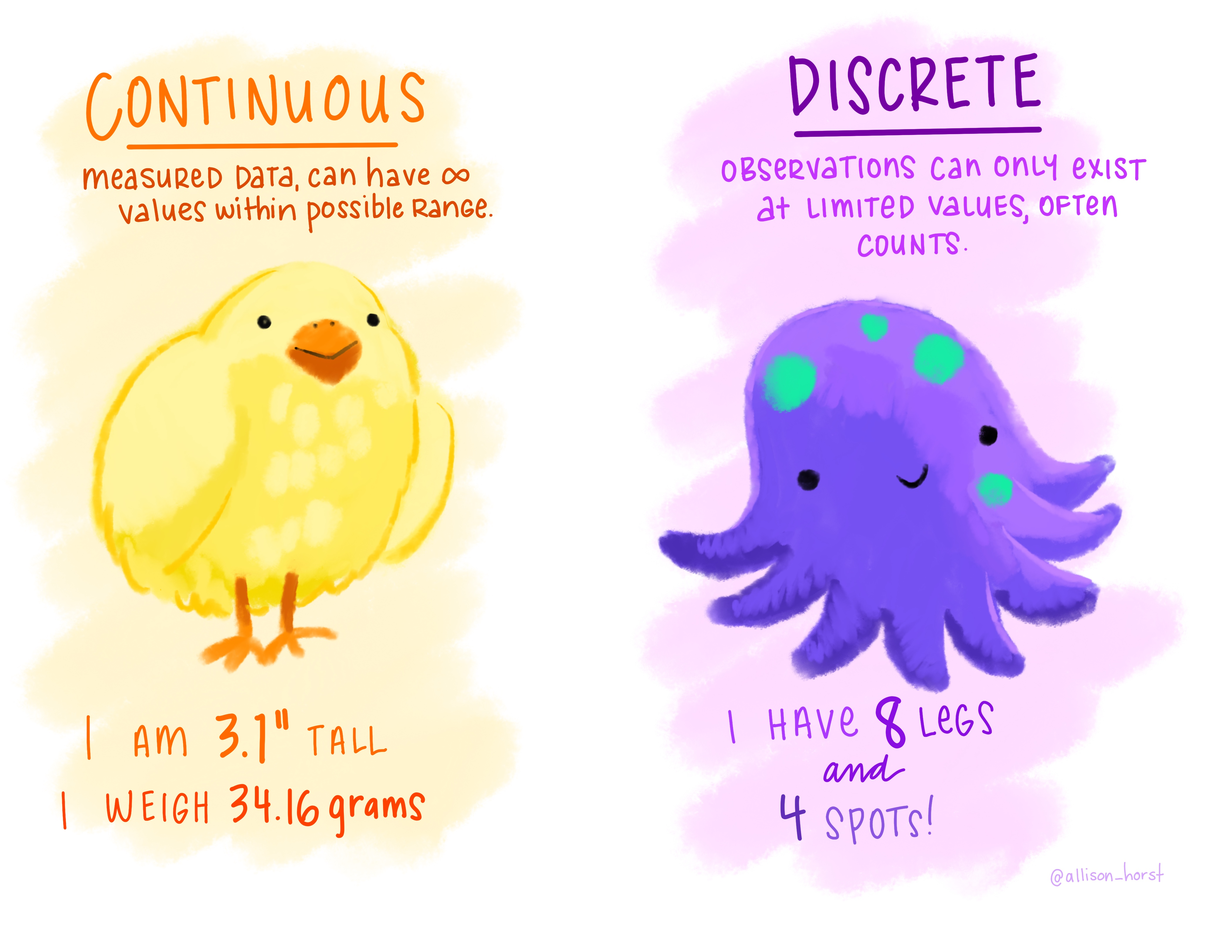
R Data Types:

Continuous: numeric
Discrete: integer or numeric (e.g., counts like number of cats)

Categorical data (next slide) are often stored as factors – we’ll cover these in a coming lecture.

Artwork by @allison_horst

Variable Types (cont.)

Sometimes data are non-numeric and store words. Even when that is the case, the data can be conveying different information.

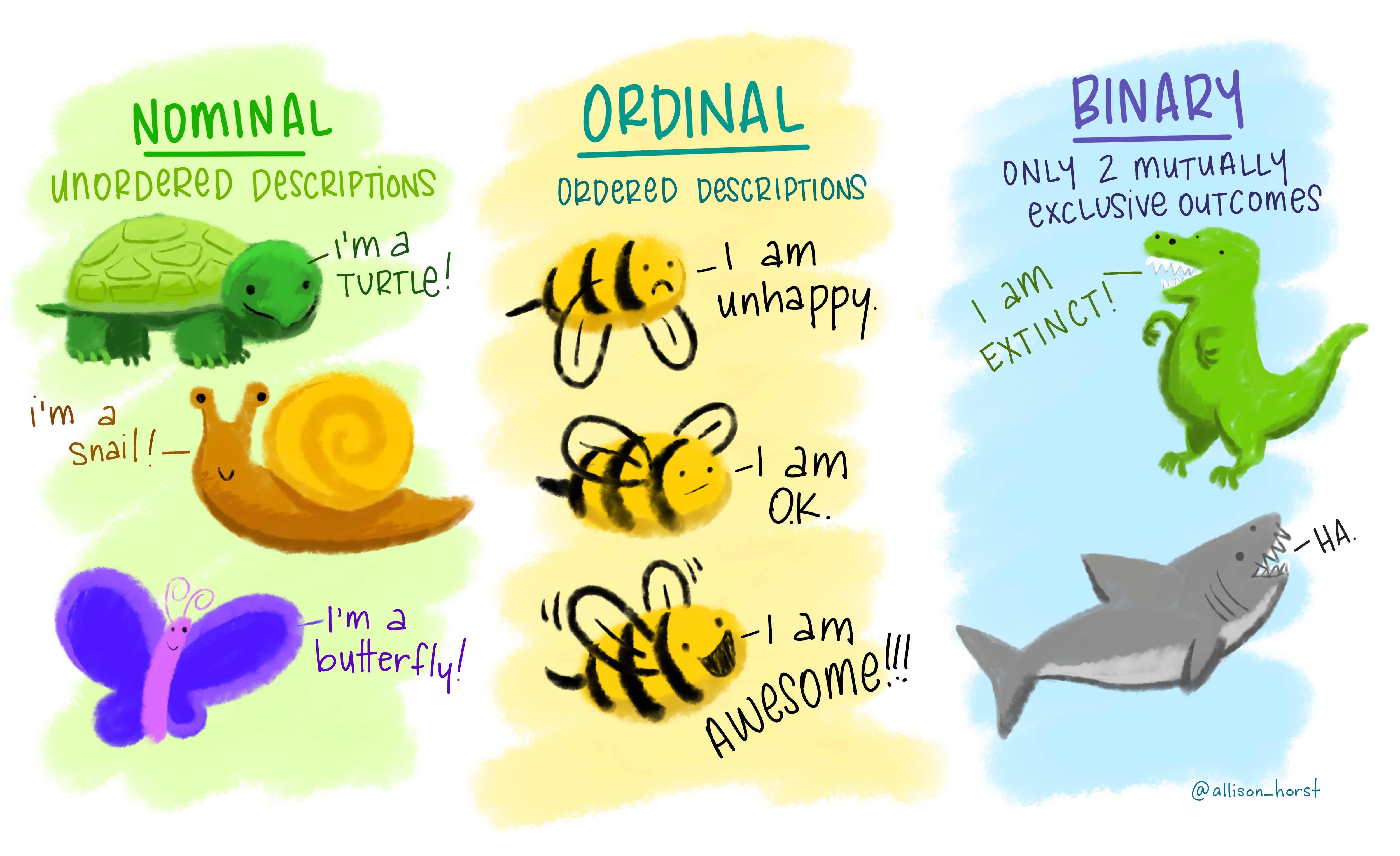
R Data Types:

Nominal: character
Ordinal: factors
Binary: logical OR numeric OR factors

Artwork by @allison_horst

Example: Cat lovers

A survey asked respondents their name and number of cats. The instructions said to enter the number of cats as a numerical value.

. . .

🚨 There is code ahead that we’re not going to discuss in detail today, but we will in coming lectures.

cat_lovers <- read_csv("https://raw.githubusercontent.com/COGS137/datasets/main/cat-lovers.csv")

The Data

cat_lovers |>
  datatable()

The Question

How many respondents have a below average number of cats?

. . .

Giving it a first shot…

cat_lovers |>
  summarise(mean = mean(number_of_cats))

Warning: There was 1 warning in `summarise()`.
ℹ In argument: `mean = mean(number_of_cats)`.
Caused by warning in `mean.default()`:
! argument is not numeric or logical: returning NA

# A tibble: 1 × 1
   mean
  <dbl>
1    NA

. . .

💡 maybe there is missing data in the number_of_cats column!

Oh why will you still not work??!!

cat_lovers |>
  summarise(mean_cats = mean(number_of_cats, na.rm = TRUE))

Warning: There was 1 warning in `summarise()`.
ℹ In argument: `mean_cats = mean(number_of_cats, na.rm = TRUE)`.
Caused by warning in `mean.default()`:
! argument is not numeric or logical: returning NA

# A tibble: 1 × 1
  mean_cats
      <dbl>
1        NA

. . .

💡 What is the type of the number_of_cats variable?

Take a breath and look at your data

. . .

glimpse(cat_lovers)

Rows: 60
Columns: 3
$ name           <chr> "Bernice Warren", "Woodrow Stone", "Willie Bass", "Tyro…
$ number_of_cats <chr> "0", "0", "1", "3", "3", "2", "1", "1", "0", "0", "0", …
$ handedness     <chr> "left", "left", "left", "left", "left", "left", "left",…

Let’s take another look

Sometimes you need to babysit your respondents

cat_lovers |>
  mutate(number_of_cats = case_when(name == "Ginger Clark" ~ 2,
                                    name == "Doug Bass" ~ 3,
                                    .default = as.numeric(number_of_cats)))

Warning: There was 1 warning in `mutate()`.
ℹ In argument: `number_of_cats = case_when(...)`.
Caused by warning in `vec_case_when()`:
! NAs introduced by coercion

# A tibble: 60 × 3
   name           number_of_cats handedness
   <chr>                   <dbl> <chr>     
 1 Bernice Warren              0 left      
 2 Woodrow Stone               0 left      
 3 Willie Bass                 1 left      
 4 Tyrone Estrada              3 left      
 5 Alex Daniels                3 left      
 6 Jane Bates                  2 left      
 7 Latoya Simpson              1 left      
 8 Darin Woods                 1 left      
 9 Agnes Cobb                  0 left      
10 Tabitha Grant               0 left      
# ℹ 50 more rows

. . .

⚠️ Notice the warning: as.numeric() couldn’t convert some values (the text answers) to numbers, so it made them NA. That’s R telling you your data had text in it! Here, case_when() replaces those rows, so it’s safe.

Always respect (& check!) data types

cat_lovers |>
  mutate(number_of_cats = case_when(name == "Ginger Clark" ~ 2,
                                    name == "Doug Bass" ~ 3,
                                    .default = as.numeric(number_of_cats))) |>
  summarise(mean_cats = mean(number_of_cats))

# A tibble: 1 × 1
  mean_cats
      <dbl>
1     0.817

Now that we know what we’re doing…

cat_lovers <- cat_lovers |>
  mutate(number_of_cats = case_when(name == "Ginger Clark" ~ 2,
                                    name == "Doug Bass" ~ 3,
                                    .default = as.numeric(number_of_cats)))

… store your data in a variable (here we’re overwriting the old cat_lovers tibble).

Answering the question

How many respondents have a below average number of cats?

cat_lovers |>
  filter(number_of_cats < mean(number_of_cats)) |>
  nrow()

[1] 33

. . .

filter() keeps only the rows that meet a condition (here, a comparison operator!). More on this in a coming lecture.

Moral of the story

If your data does not behave how you expect it to, type coercion upon reading in the data might be the reason.
Go in and investigate your data, apply the fix, save your data, live happily ever after.

Recap

Always best to think of data as part of a tibble
- This plays nicely with the tidyverse as well
- Rows are observations, columns are variables
What are the common variable types in R
- How do I create a variable of each type?
- When would I use each one?
What is a vector, and why must its values all be the same type?
Do I know how to determine the class/type of a variable?
Can I explain dynamic typing? How is it different from coercion?
Can I operate on variables and values using…
- arithmetic operators?
- comparison operators?
- logical operators?
What does NA do in a calculation, and how do I handle it?
What are dataframes/tibbles? and why are they useful?
What is the difference between installing and loading a package?